本文首发于微信公众号《与有三学AI》

[caffe解读] caffe从数学公式到代码实现4-认识caffe自带的7大loss

本节说caffe中常见loss的推导，具体包含下面的cpp。

multinomial_logistic_loss_layer.cppsoftmax_loss_layer.cppeuclidean_loss_layer.cppsigmoid_cross_entropy_loss_layer.cppcontrastive_loss_layer.cpphinge_loss_layer.cppinfogain_loss_layer.cpp

1 multinomial_logistic_loss_layer.cpp

数学定义

x是输入，y是label，l是loss

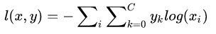
上述式只有当样本i属于第k类时，

 yk=1，其他情况 ,yk=0，我们计不为0的 yk =y。

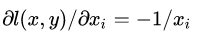
forward & backward

forward对所有 Xi求和，注意，此处没有对图像维度的像素进行归一化，只对batch size维度进行归一化，num就是batch size，这与下面的softmaxlosslayer是不一样的。

void MultinomialLogisticLossLayer::Forward_cpu(

const vector*>& bottom, const vector*>& top) {

const Dtype* bottom_data = bottom[0]->cpu_data();

const Dtype* bottom_label = bottom[1]->cpu_data();

int num = bottom[0]->num();

int dim = bottom[0]->count() / bottom[0]->num();

Dtype loss = 0;

for (int i = 0; i < num; ++i) {

int label = static_cast(bottom_label[i]);

Dtype prob = std::max( bottom_data[i * dim + label], Dtype(kLOG_THRESHOLD));

loss -= log(prob);

}

top[0]->mutable_cpu_data()[0] = loss / num;

}

backward可以自己去看，很简单就不说了

2 softmax_layer.cpp

数学定义

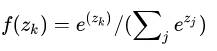
softmax是我们最熟悉的了，分类任务中使用它，分割任务中依然使用它。Softmax loss实际上是由softmax和cross-entropy loss组合而成，两者放一起数值计算更加稳定。

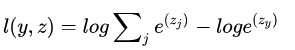
令z是softmax_with_loss层的输入，f(z)是softmax的输出，则

单个像素i的softmax loss等于cross-entropy error如下

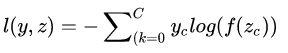
展开上式：

在网络中，z是即bottom blob，l(y,z)是top blob,反向传播时，就是要根据top blob diff得到bottom blob diff，所以要得到 

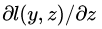
下面求loss对z的第k个节点的梯度

可见，传给groundtruth label节点和非groundtruth label是的梯度是不一样的。

forward就不看了，看看backward吧。

Dtype* bottom_diff = bottom[0]->mutable_cpu_diff();

const Dtype* prob_data = prob_.cpu_data();

caffe_copy(prob_.count(), prob_data, bottom_diff);

const Dtype* label = bottom[1]->cpu_data();

int dim = prob_.count() / outer_num_;

int count = 0;

for (int i = 0; i < outer_num_; ++i) {

for (int j = 0; j < inner_num_; ++j) {

const int label_value = static_cast(label[i * inner_num_ +

j]);

if (has_ignore_label_ && label_value == ignore_label_) {

for (int c = 0; c < bottom[0]->shape(softmax_axis_); ++c) {

bottom_diff[i * dim + c * inner_num_ + j] = 0;

}

} else {

bottom_diff[i * dim + label_value * inner_num_ + j] -= 1;

++count;

}

}

}

Test_softmax_with_loss_layer.cpp

作为loss层，很有必要测试一下，测试也分两块，forward和backward。

Forward测试是这样的，定义了个bottom blob data和bottom blob label，给data塞入高斯分布数据，给label塞入0～4。

blob_bottom_data_(new

Blob<Dtype>(10, 5, 2, 3)),

blob_bottom_label_(new

Blob<Dtype>(10, 1, 2, 3)),

然后分别ingore其中的一个label做5次，最后比较，代码如下。

Dtype accum_loss = 0;

for (int label = 0; label < 5; ++label) {

layer_param.mutable_loss_param()->set_ignore_label(label);

layer.reset(new SoftmaxWithLossLayer<Dtype>(layer_param));

layer->SetUp(this->blob_bottom_vec_,

this->blob_top_vec_);

layer->Forward(this->blob_bottom_vec_, this->blob_top_vec_);

accum_loss += this->blob_top_loss_->cpu_data()[0];

}

// Check that each label was included all but

once.

EXPECT_NEAR(4 * full_loss, accum_loss, 1e-4);

至于backwards，直接套用checker.CheckGradientExhaustive就行，它自己会利用数值微分的方法和你写的backwards来比较精度。

TYPED_TEST(SoftmaxWithLossLayerTest,

TestGradientIgnoreLabel) {

typedef typename TypeParam::Dtype Dtype;

LayerParameter layer_param;

//

labels are in {0, ..., 4}, so we'll ignore about a fifth of them

layer_param.mutable_loss_param()->set_ignore_label(0);

SoftmaxWithLossLayer<Dtype> layer(layer_param);

GradientChecker<Dtype> checker(1e-2, 1e-2, 1701);

checker.CheckGradientExhaustive(&layer, this->blob_bottom_vec_,

this->blob_top_vec_, 0);

}

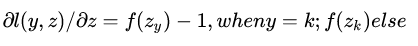
3 eulidean_loss_layer.cpp

euclidean loss就是定位检测任务中常用的loss。 

数学定义：

forward & backward

void EuclideanLossLayer<Dtype>::Backward_cpu(const

vector<Blob<Dtype>*>& top,

const vector<bool>& propagate_down, const

vector<Blob<Dtype>*>& bottom) {

for (int i = 0; i < 2; ++i) {

if (propagate_down[i]) {

const Dtype sign = (i == 0) ? 1 : -1;

const Dtype alpha = sign * top[0]->cpu_diff()[0] / bottom[i]->num();

caffe_cpu_axpby( bottom[i]->count(),  // count

alpha, // alpha

diff_.cpu_data(), // a

Dtype(0), // beta

bottom[i]->mutable_cpu_diff()); // b

}

}

}

testcpp就不说了。

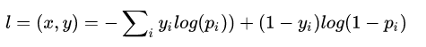
4 sigmoid_cross_entropy_loss_layer.cpp

与softmax loss的应用场景不同，这个loss不是用来分类的，而是用于预测概率，所以在loss中，没有类别的累加项。

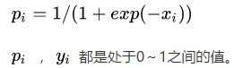
令第i个节点输入 Xi，输出总loss为l，label为 yi，则loss定义如下

其中

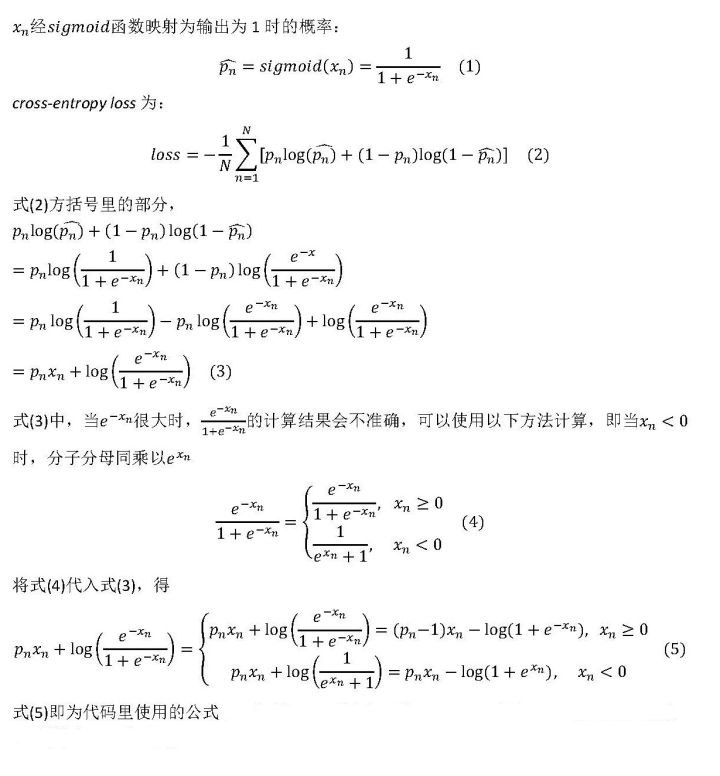
上式子有个等价转换，这是为了更好的理解caffe 中forward的计算，公司太多我就直接借用了，如果遇到了原作者请通知我添加转载申明。

http://blog.csdn.net/u012235274/article/details/51361290

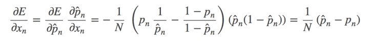
反向求导公式如下：

在经过上面的转换后，避开了数值计算不稳定的情况，caffe中的源码是对整个的bottom[0]->count进行计算累加的，没有区分label项。

for (int i = 0; i < bottom[0]->count(); ++i) {

const int target_value = static_cast<int>(target[i]);

if (has_ignore_label_ && target_value == ignore_label_) {

continue;

}

loss -= input_data[i] * (target[i] - (input_data[i] >= 0)) - log(1 + exp(input_data[i] - 2 * input_data[i] * (input_data[i] >= 0)));

++valid_count;

}

反向传播很简单就不看了

5 contrastive_loss_layer.cpp

有一类网络叫siamese network，它的输入是成对的。比如输入两张大小相同的图，网络输出计算其是否匹配。所采用的损失函数就是contrastive loss

数学定义：

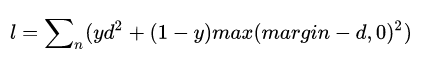
d就是欧氏距离，y是标签，如果两个样本匹配，则为1，否则为0. 当y=1，loss就是欧氏距离，说明匹配的样本距离越大，loss越大。当y=0，是，就是与阈值margin的欧式距离，说明不匹配的样本，欧氏距离应该越大越好，超过阈值最好，loss就等于0.

反向传播其实就是分y=1和y=0两种情况下的euclidean loss的反向传导，由于与euclidean

loss非常相似，不再赘述。

6 hinge_loss_layer.cpp

这是一个多分类的loss, 也是SVM的目标函数，没有学习参数的全连接层InnerProductLayer+HingeLossLayer就等价于SVM。

数学定义

这个层的输入bottom[0]是一个N*C*H*W的blob，其中取值任意值，label就是N*1*1*1，其中存储的就是整型的label{0,1,2,…,k}。

相当于SVM中的 

参考博客http://blog.leanote.com/post/braveapple/Hinge-Loss-%E7%9A%84%E7%90%86%E8%A7%A3

假如预测类别数是K个，正确的label是M，预测值为 

 ，即是第n个样本对第k类的预测值，那么当k=M时,

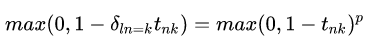
当k!=M时，

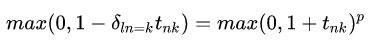
其中p=1，p=2分别对应L1范数和L2范数，以L1为例

Forward

caffe_copy(count, bottom_data, bottom_diff);

for (int i = 0; i < num; ++i) { bottom_diff[i * dim + static_cast<int>(label[i])] *= -1;

}

for (int i = 0; i < num; ++i) {

for (int j = 0; j < dim; ++j) {

bottom_diff[i * dim + j] = std::max( Dtype(0), 1 + bottom_diff[i * dim + j]);

}

}

Dtype* loss = top[0]->mutable_cpu_data();

switch (this->layer_param_.hinge_loss_param().norm()) {

case HingeLossParameter_Norm_L1:

loss[0] = caffe_cpu_asum(count, bottom_diff) / num; break;

case HingeLossParameter_Norm_L2:

loss[0] = caffe_cpu_dot(count, bottom_diff, bottom_diff) / num; break;

default: LOG(FATAL) << "Unknown Norm";

}

只需要根据上面的转化后的式子，在正确label处乘以-1，然后累加即可。

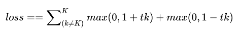
再看反向梯度求导：

当进行一次forward之后，

bottom_diff=

[max(0,1+t0),max(0,1+t1),...,max(0,1−tk),...,

max(0,1−tK-1)]

我们现在要求梯度，期望是1+tk>0时为1，1-tk>0时为-1，其他情况为0，

当任意一项1+tk或者1-tk<0时，会有梯度=0。实际上就是求上面向量各自元素的符号，当1+tk>0，sign(1+tk)，只是max(0,1−tk)这个应该反过来，当1-tk>0时，sign(tk-1)=-1。

代码如下：

Dtype* bottom_diff = bottom[0]->mutable_cpu_diff();

const Dtype* label = bottom[1]->cpu_data();

int num = bottom[0]->num();

int count = bottom[0]->count();

int dim = count / num;

for (int i = 0; i < num; ++i) {

bottom_diff[i * dim + static_cast(label[i])] *= -1;

}

const Dtype loss_weight = top[0]->cpu_diff()[0];

switch (this->layer_param_.hinge_loss_param().norm()) {

case HingeLossParameter_Norm_L1:

caffe_cpu_sign(count, bottom_diff, bottom_diff);

caffe_scal(count, loss_weight / num, bottom_diff);

break;

case HingeLossParameter_Norm_L2:

caffe_scal(count, loss_weight * 2 / num, bottom_diff);

break;

default: LOG(FATAL) << "Unknown Norm";

}

}

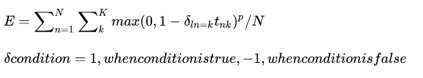
7 infogain_loss_layer.cpp

数学定义：

输入bottom_data是N*C*H*W维向量，bottom_label是N*1*1*1维向量，存储的就是类别数。它还有个可选的bottom[2]，是一个infogain matrix矩阵,它的维度等于num_of_label * num_of_label。每个通道c预测的是第c类的概率，取值0～1，所有c个通道的概率相加=1。是不是像soft Max？

实际上它内部就定义了shared_ptr > softmax_layer_，用于映射输入。

Loss定义如下：

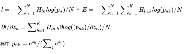
 代表H的第ln行，K是所有类别数，如果H是一个单位矩阵，那么只有对角线有值，回到文章开头，这就是multinomial_logistic_loss_layer。当H是一个普通矩阵时，当groundtruth label为k，

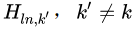
 时，值也可以非零。这样各个类别之间就不存在竞争关系了，后来的mask-rcnn中实际上loss也就是去除了这重竞争关系。

Forward：

void InfogainLossLayer<Dtype>::Forward_cpu(const vector<Blob<Dtype>*>& bottom,

const vector<Blob<Dtype>*>& top) {

softmax_layer_->Forward(softmax_bottom_vec_, softmax_top_vec_);

const Dtype* prob_data = prob_.cpu_data();

const Dtype* bottom_label = bottom[1]->cpu_data();

const Dtype* infogain_mat = NULL;

if (bottom.size() < 3) { infogain_mat = infogain_.cpu_data();

} else { infogain_mat = bottom[2]->cpu_data();}

int count = 0;

Dtype loss = 0;

for (int i = 0; i < outer_num_; ++i) {

for (int j = 0; j < inner_num_; j++) {

const int label_value = static_cast(bottom_label[i * inner_num_ + j]);

if (has_ignore_label_ && label_value == ignore_label_) {continue;}

DCHECK_GE(label_value, 0);

DCHECK_LT(label_value, num_labels_);

for (int l = 0; l < num_labels_; l++)

{  loss -= infogain_mat[label_value * num_labels_ + l] * log(std::max( prob_data[i * inner_num_*num_labels_ + l * inner_num_ + j],

Dtype(kLOG_THRESHOLD)));}

++count; } }

top[0]->mutable_cpu_data()[0] = loss / get_normalizer(normalization_, count);

if (top.size() == 2) { top[1]->ShareData(prob_); }}

上面与multinomial_logistic_loss_layer的区别就在于每一项乘了infogain_mat[label_value *

num_labels_ + l]。

Backward:

for (int l = 0; l < num_labels_; ++l) {

    bottom_diff[i * dim + l * inner_num_ + j] = prob_data[i*dim + l*inner_num_ + j]*sum_rows_H[label_value] - infogain_mat[label_value * num_labels_ + l];

  }

这个，看了4篇了大家不妨自己推一推？不行咱再一起来

更多请移步

1，我的gitchat达人课

龙鹏的达人课​

2，AI技术公众号,《与有三学AI》

一文说说这十多年来计算机玩摄影的历史​

3，以及摄影号，《有三工作室》

冯小刚说，“他懂我”